Notes on RL
Published:
These are personal notes on reinforcement learning, mainly based on the content of the UC Berkeley course thaught by Sergey Levine.
Main goal in reinforcement learning
The main optimization problem that reinforcement learning tries to tackle is maximizing the expected reward along a time horizon $T$ (where $T$ could be $\infty$) in a Markov Decision Process (MDP), w.r.t. the policy parameters $\theta$.
\[\theta^\star = \text{argmax}_\theta \mathbb{E}_{\tau\sim p_{\theta}(\tau)} \left[ \sum_t r(s_t, a_t) \right] = \text{argmax}_\theta J(\theta)\] \[p_\theta(s_1, a_1, \dots, s_T, a_T) = p(s_1) \prod_{t=1}^T \pi_\theta(a_t | s_t) p(s_{t+1} | s_t, a_t)\]where $ \pi_\theta (a_t | s_t) $ is the policy in the MDP and $ p(s_{t+1} | s_t, a_t) $ is the transition function (or dynamics) of the environment (system).
In the finite horizon case ($T$ finite) the expectation is taken w.r.t the state-action marginal $p_\theta(s_t,a_t)$, thus we seek to maximize the following optimization problem. This is called the undiscounted average reward.
\[\theta^\star = \text{argmax}_\theta \frac{1}{T} \sum_{t=1}^T \mathbb{E}_{ (s_t, a_t) \sim p_{\theta}(s_t, a_t)} \left[ r(s_t, a_t) \right]\]Anatomy of a RL problem
Normally reinforcement learning problems have a similar three step structure.
- Sample generation: Interact with the world to get tuples of the form $\zeta=(s_{t+1}, s_t, a_t, r_t)$
- Estimating return / Fitting a model: In the case of model-free RL we might just estimate the cumulative reward of each trajectory. In model-based RL it is common to fit models of the dynamics of the environment.
- Policy improvement : This could be a simple update step like gradient descent
Common definitions in RL
Q-functions are commonly used in RL algorithms, they represent the total expected reward from taking action $a_t$ and state $s_t$ from $t$ up to $T$. This function could be estimated by sampling an environment and retrieving tuples $\zeta$
\[Q^\pi(s_t, a_t) = \sum_{t'=t}^T \mathbb{E}_{\pi_\theta}\left[ r(s_{t'}, a_{t'}) | s_t, a_t \right] \\ Q^\pi(s_t, a_t) = r(s_t, a_t) + \mathbb{E}_{s_+ \sim p(s_{t+1}|s_t, a_t)}[V^\pi (s_{t+1})]\]Value functions are also commonly used and they are degined as the total reward from taking action $s_t$ from $t’$ to $T$.
\[V^\pi(s_t) = \sum_{t'=t}^T \mathbb{E}_{\pi_\theta}\left[ r(s_{t'}, a_{t'}) | s_t \right] \\ V^\pi(s_t) = \sum_{t'=t}^T \mathbb{E}_{a_t \sim \pi_\theta}\left[ Q^\pi(s_t, a_t) \right]\]Recall that optimizing the expected value function is equivalent to maximizing the main RL objective. Note: If $Q_{s,a} > V_{s}$ means that your policy is better than average.
The advantage function $A^\pi(s_t, u_t)$ quantifies how good an action is, if the quantity is positive action $a_t$ is better than average and negative otherwise.
\[A^\pi(s_t, a_t) = Q^\pi(s_t, a_t) - V^\pi(s_t)\]Types of RL algorithms
- Policy gradients: directly optimize the main goal in RL described above. examples: REINFORCE, Policy Gradient, Trust Region Policy Optimization
- Value-based: estimate value function or Q-function (no explicit policy). examples: Q-learning, DQN , Temporal difference learning, Value Iteration
- Actor-Critic: estimate value function or Q-function of the current policy and improve the policy examples:: Asynchronous advantage actor-critic (A3C), Soft actor-critic (SAC)
- Model-based RL: learn the transition model and then use it for planning or to train a policy examples: Dyna, Guided policy search
Policy gradient methods:
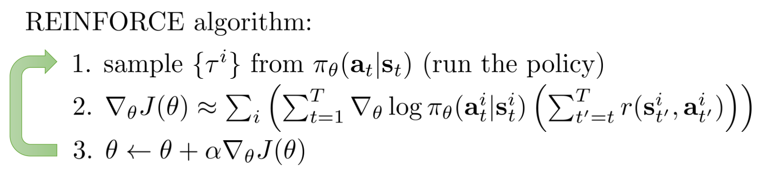
REINFORCE is a model-free reinforcement learning algorithm that uses on-policy data to estimate a gradient of our policy $\pi_\theta$ by using an estimate of the cumulative reward gotten from the on-policy data. For more information about the derivation of the policy gradient algorithm, you can check the courses notes. The PG algorithm lets us estimate the gradient of our policy without the need of knowing the full trajectory distribution $p(\tau)$. The algorithm computes the following gradient
\[\nabla_\theta J(\theta) = \mathbb{E}_{\tau \sim p_\theta(\tau)} \left[ \left( \sum_t^T \nabla_\theta \log \pi_\theta(a_t| s_t) \right)\left( \sum_t^T r(s_t, a_t)\right) \right] \approx \frac{1}{N} \sum_n^N \left[ \dots \right]\]We can use this estimate to update out policy via a standard gradient descent $\theta^+ = \theta + \alpha \nabla_\theta J(\theta)$. Remember that the values for computing this estimate come from the MDP tuple $\zeta$. One intuition is that the first term gives you the direction to steer the policy to a certain action $a_t$ which is sampled form the environment, and the second term gives you the weighting of this specific gradient towards $a_t$. For example, actions that yield better reward are gonna contribute more to the gradient than actions that give lower reward.
NOTE: This algorithm also works with partial observability, $\pi$ could be conditioned on $o_t$ instead of $s_t$.
Variance reduction tricks
Given that a certain action $a_t$ can’t affect past rewards we can change the above equation by this more commonly implemented variant, by:
\[\nabla_\theta J(\theta) \approx \frac{1}{N} \sum_n^N \left[ \sum_{t=1}^T \nabla_\theta \log \pi_\theta(a_t| s_t) \left( \sum_{t'=t}^T \gamma^{(t'-t)} r(s_{t'}, a_{t'})\right) \right] \\ \approx \frac{1}{N} \sum_n^N \left[ \sum_{t=1}^T \nabla_\theta \log \pi_\theta(a_t| s_t) \hat{Q} \right] \\\]where $\gamma$ is the typical discount factor (usually $0.99$). In the case that we do not have well-behaved rewards (gaussian-like rewards), we need to recenter this rewards using a baseline (this baseline won’t change the expected value of our gradient. This baseline $b$ is in practice an average reward over all samples.
\[\nabla_\theta J(\theta) \approx \frac{1}{N} \sum_n^N \left[ \sum_{t=1}^T \nabla_\theta \log \pi_\theta(a_t| s_t) \left( \left( \sum_{t'=t}^T \gamma^{(t'-t)} r(s_{t'}, a_{t'}) \right) - b \right) \right]\]We can also modify the algorithm to use the true expected reward-to-go $Q^\pi(s_t, a_t)$, as a baseline we can average these rewards to go using an empirical estimate. This empirical estimate is an approximation of the value function $V^\pi(s_t)$ as seen before.
\[\nabla_\theta J(\theta) \approx \frac{1}{N} \sum_n^N \left[ \sum_{t=1}^T \nabla_\theta \log \pi_\theta(a_t| s_t) \left(Q^\pi(s_t, a_t) - V_\pi(s_t)\right) \right] \\ \approx \frac{1}{N} \sum_n^N \left[ \sum_{t=1}^T \nabla_\theta \log \pi_\theta(a_t| s_t) A^\pi(s_t, a_t) \right] \\\]The better estimate of $A^\pi$ the lower the variance of out gradient.
Off-policy policy gradient
PG is an on-policy algorithm, thus it needs samples $\zeta^\pi$ drawn from the policy $\pi$. We could deriva an off-policy variant by using importance sampling. Importance sampling lets you estimate an expectation over a distribution $p $by sampling from an auxiliary distribution $q$.
\[\mathbb{E}_{x \sim p(x)} \left[ f(x) \right]= \mathbb{E}_{x \sim q(x)}\left[ \frac{p(x)}{q(x)} f(x) \right]\]The full derivation of the off-policy PG method can be seen in the video lecture. The gradient estimate looks as follows.
\[\nabla_\theta J(\theta) \approx \frac{1}{N} \sum_n^N \left[ \sum_{t=1}^T \frac{\pi_{\theta}(a_t | s_t)}{\pi_{\theta_{old}}(a_t |s_t)} \nabla_\theta \log \pi_\theta(a_t| s_t) \hat{Q} \right]\]This will help us use information from the replay buffer that does not belong to the most recent policy. We would also need to save the probability $\pi_{\theta_{old}}$ in the replay buffer for later use.
Implementation details:
To code this up, we can code a pseudo loss-function which gradient is the policy gradient, we can then compute this using a standard autodiff package like pytorch. The loss-function would look like this and it is basically a weighted ML by the Q values.
\[\bar{J}(\theta) = \frac{1}{N} \sum_n^N \left[ \sum_{t=1}^T \log \pi_\theta(a_t| s_t) \hat{Q}\right]\]NOTES: Gradients are very noisy so use large batch sizes, low learning rate, tricky to tune.
Estimating value functions for Actor-Critic methods
We can estimate a value function by getting a single sample estimate of our reward (in the case of single sample, it is the same as the estimate of the reward function). $V^\pi(s_t) \approx \sum_t r(s_t, a_t)$. We can use this estimate to train a neural network using Stochastic Gradient Descent (SGD) via the following loss function. $\mathcal{L}_2$ function is incorrect because it uses the previous estimate of $V^\pi$ but it works better in practice than just optimizing the empirical estimate $\mathcal{L}_1$.
\[\mathcal{L}_1(\phi) = \frac{1}{2} \sum_i \| \hat{V}_\phi^\pi(s_i) - \sum_t r(s_t, a_t) \|^2 \\ \mathcal{L}_2(\phi) = \frac{1}{2} \sum_i \| \hat{V}_\phi^\pi(s_i) - \left(r(s_i, a_i) + \gamma V^{\pi}_{\phi_{old}} (s_{t+1}) \right) \|^2\]$V_{\phi_{old}}$ in practice it just evaluates the next states $s_{t+1}$ using the value network. This should not be added to the computation graph for the autodiff. An actor-critic algorithm works like follows and it basically trains a value function on the go.
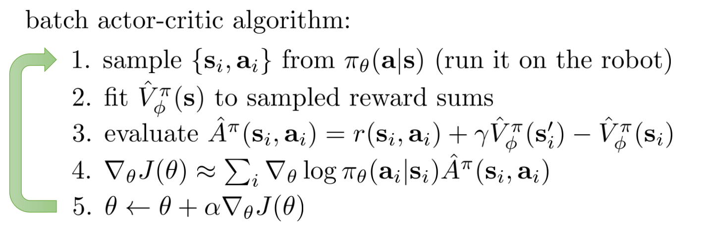
Actor critic methods have lower variance than normal policy gradient but they are not unbiased. PG is unbiased but maybe tricky to train because it can have a huge variance.
\[\nabla_\theta J(\theta) \approx \frac{1}{N} \sum_n^N \left[ \sum_{t=1}^T \nabla_\theta \log \pi_\theta(a_t| s_t) (r(s_t, a_t) + \gamma \hat{V}_\phi^\pi(s_{t+1}) - \hat{V}_\phi^\pi(s_t) ) \right] \\ \nabla_\theta J(\theta) \approx \frac{1}{N} \sum_n^N \left[ \sum_{t=1}^T \nabla_\theta \log \pi_\theta(a_t| s_t) (\sum_{t'=t} \gamma^{t' - t} r(s_t, a_t) - V^\pi(s_t) ) \right]\]The first equation is the actor critic gradient, the second equation is using the value function estimate as a state dependent baseline, this will have no bias and lower variance. We can also combine these two by estimating the cumulative rewards until a fixed time horizon $t+n$.
\[\hat{A}_n^\pi (s_t, a_t) = \sum_{t'=t}^{t+n} \gamma^{t' - t} r(s_{t'}, a_{t'}) + \gamma^n \hat{V}_\phi^\pi (s_{t+n}) - \hat{V}_\phi^\pi(s_t)\]The second terms approximated the tail of the value and the third term centers the total reward
Generalized advantage estimation
We can create a weighted average of $\hat{A}_n^\pi$ estimators and weight them by $\lambda^{n-1}$ because we want estimates with lower variance (therefore weight more estimates with lower $n$) (Note that $\lambda < 1$). We therefore get the following advantage estimate
\[\hat{A}_{GAE}^\pi(s_t, a_t) = \sum_{n}^\infty \lambda^{n-1}\hat{A}_n^\pi(s_t, a_t) \\ \hat{A}_{GAE}^\pi(s_t, a_t) = \sum_{t'=t}^\infty (\gamma\lambda)^{t'-t}(r(s_{t'}, a_{t'}) + \gamma \hat{V}_\phi^\pi(s_{t'+1}) - \hat{V}_\phi^\pi(s^{t'}))\]This could be seen as a combination of Monte Carlo reward samples and the use of function approximation like in standard actor-critic. $\lambda$ then serves as a hyperparameter to tradeoff between bias and variance. The lower $\lambda$ the faster we will forget about the higher $n$ advantages and this gives us a lower variance but higher bias. If $\lambda \approx 1$ we are gonna care a lot about the sampled rewards and this is gonna increase the variance but also lower our bias.
Value-function methods
The following section will explore value function methods, these do not have a policy (actor), they learn the critic dicrecly.
Fitted value iteration algorithm
Because of the course of dimensionality we cannot learn a tabular value function of reasonably big dimensionaliy using standard value and policy iteration (VI and PI). We can learn a value function with a neural network by doing “Fitted value itration”. This algorithm has two steps and they are repeated until the value function is learned
\[Q^\pi(s, a) = r(s, a) + \gamma \mathbb{E}_{s'}[V_\phi(s')]\\ \phi^* = \text{argmax}_\phi \frac{1}{2} \sum_i \| \hat{V}_\phi^\pi(s_i) - \text{max}_aQ^\pi(s_t, a_t) \|^2\]Bare in mind that this assummes that the transition dynamics are known and we can enumerate all the actions for every step we sample.
Remarks:
- Tabular VI always converge because it is a contraction w.r.t. $\infty$ norm
- Fitted VI dos not converge because there is a contraction w.r.t. $l_2$ norm (The square loss) after the Bellman-update contraction. Unfortunately these contractions do not compose and it could be that you diverge.
Fitted Q iteration algorithm
This algorithm will not require us to know the system dynamics to be able to compute the expectation of the value function (reward to go) from the next time step.
\[y_i = r(s, a) + \gamma \mathbb{E}[V_\phi(s')] \approx r(s, a) + \gamma \text{max}_{a'}Q_\phi(s', a')\\ \phi^* = \text{argmax}_\phi \frac{1}{2} \sum_i \| \hat{Q}_\phi^\pi(s_i, a_i) - y_i \|^2\]In this method we do not need to enumerate all actions but we need a way to optimize the function, $max_{a’}Q_\phi(s’, a’)$.
Remarks:
- Fitted Q iteration is an off-policy algorithm because it just makes the assumption that your policy s the $\text{argmax}$ policy
- Does not require knowledge of the transition function $T_{ij}$, it just uses evaluations of the $Q_\phi$ function estimate.
- If we run this in an online fashion by taking single transitions and single gradient steps we are doing Q-learning
- Same contraction problems as with fitted VI
Fixing Q learning
There is a problem with Q learning, the target that we are trying to use are always moving with each iteration, additionaly our samples are not i.i.d. We can fix the problem of not i.i.d samples by creating a dataset called a “replay buffer” from this buffer we can sample batches to train our neural network.
The second problem can be fixed by having auxiliary neural network parameters $\phi’$ and updating this every $N$ steps or slowly by poliak averaging $\phi’ \leftarrow \tau \phi’ + (1-\tau)\phi$, this just updates the parameters very slowly, usually $\tau = 0.999 $. The algorithm works as follows and it is called DQN if we update the parameters every $N$ steps.

To extedn Q-learning to continuous action spaces we can use stochastic optimization like CEM or CMA-ES to maximize $max_{a’} Q(s’, a’)$. We can also represent an easily maximizable Q function that is quadratic in the actions but complicated in the state (This is called Normalized Advantage Functions), the max of this function is simply the value function $V_\phi(s)$
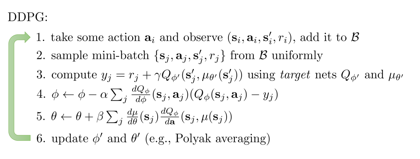
\[Q_\phi(s_t, a_t) = -\frac{1}{2}(a -\mu_\phi(s))^T P_\phi(s)(a - \mu_\phi(s)) + V_\phi(s)\]DDPG (Deep Deterministic Policy Gradients) (Off-Policy)
Another option is to use DDPG which learns to optimize $Q(s’,\text{argmax}_{a’}Q(s’, a’))$ by learning a neural network that estimates this $\text{argmax}$. The gradients for this network are computed using the chain rule